Exploratory data analysis is an essential stage in any data science project. It allows you to become familiar with the data you are working with while also to identify potential strategies for progressing the project and flagging any areas of concern.
In this chapter we will look at three different perspectives on exploratory data analysis: its purpose for you as a data scientist, its purpose for the broader team working on the project and finally its purpose for the project itself.
8.2 Get to know your data
Let’s first focus on an exploratory data analysis from our own point of view, as data scientists.
Exploratory data analysis (or EDA) is a process of examining a data set to understand its overall structure, contents, and the relationships between the variables it contains. EDA is an iterative process that’s often done before building a model or making other data-driven decisions within a data science project.
Exploratory Data Analysis: quick and simple exerpts, summaries and plots to better understand a data set.
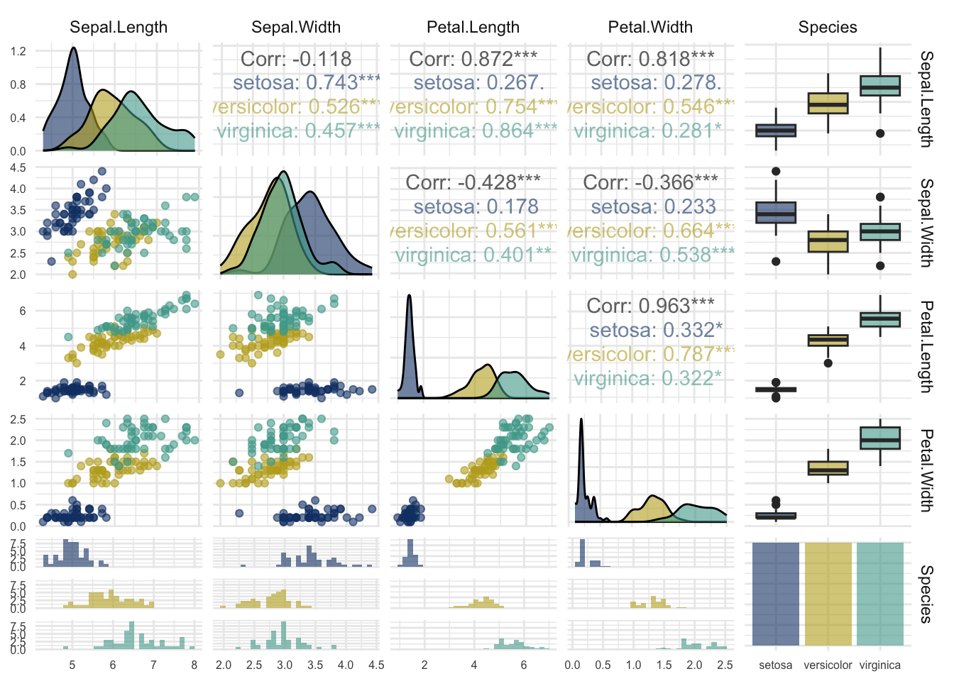
One key aspect of EDA is generating quick and simple summaries and plots of the data. These plots and summary statistics can help to quickly understand the distribution of and relationships between the recorded variables. Additionally, during an exploratory analysis you will familiarise yourself with the structure of the data you’re working with and how that data was collected.
Investigating marginal and pairwise relationships in the Iris dataset.
Since EDA is an initial and iterative process, it’s rare that any component of the analysis will be put into production. Instead, the goal is to get a general understanding of the data that can inform the next steps of the analysis.
In terms of workflow, this means that using one or more notebooks is often an effective way of organising your work during an exploratory analysis. This allows for rapid iteration and experimentation, while also providing a level of reproducibility and documentation. Since notebooks allow you to combine code, plots, tables and text in a single document, this makes it easy to share your initial findings with stakeholders and project managers.
8.3 Start a conversation
An effective EDA sets a precedent for open communication with the stakeholder and project manager.
We’ve seen the benefits of an EDA for you as a data scientist, but this isn’t the only perspective.
One key benefit of an EDA is that it can kick-start your communication with subject matter experts and project managers. You can build rapport and trust early in a project’s life cycle by sharing your preliminary findings with these stakeholders . This can lead to a deeper understanding of both the available data and the problem being addressed for everyone involved. If done well, it also starts to build trust in your work before you even begin the modelling stage of a project.
8.3.1 Communicating with specialists
Sharing an exploratory analysis will inevitably require a time investment. The graphics, tables, and summaries you produce need to be presented to a higher standard and explained in a way that is clear to a non-specialist. However, this time investment will often pay dividends because of the additional contextual knowledge that the domain-expert can provide. They have a deep understanding of the business or technical domain surrounding the problem. This can provide important insights that aren’t in the data itself, but which are vital to the project’s success.
As an example, these stakeholder conversations often reveal important features in the data generating or measurement process that should be accounted for when modelling. These details are usually left out of the data documentation because they would be immediately obvious to any specialist in that field.
8.3.2 Communicating with project manager
An EDA can sometimes allow us to identify cases where the strength of signal within the available data is clearly insufficient to answer the question of interest. By clearly communicating this to the project manager, the project can be postponed while different, better quality or simply more data are collected. It’s important to note that this data collection is not trivial and can have a high cost in terms of both time and capital. It might be that collecting the data needed to answer a question will cost more than we’re likely to gain from knowing that answer. Whether the project is postponed or cancelled, this constitutes a successful outcome for the project; the aim is to to produce insight or profit - not to fit models for their own sake.
8.4 Scope Your Project
EDA is an initial assessment of whether the available data measure the correct values, in sufficient quality and quantity, to answer a particular question.
A third view on EDA is as an initial assessment of whether the available data measure the correct values, with sufficient quality and quantity, to answer a particular question. In order for EDA to be successful, it’s important to take a few key steps.
First, it’s important to formulate a specific question of interest or line of investigation and agree on it with the stakeholder. By having a clear question in mind, it will be easier to focus the analysis and identify whether the data at hand can answer it.
Next, it’s important to make a record (if one doesn’t already exist) of how the data were collected, by whom it was collected, what each recorded variable represents and the units in which they are recorded. This meta-data is often known as a data sheet or data dictionary. Having this information in written form is crucial when adding a new collaborator to a project, so that they can understand the data generating and measurement processes, and are aware of the quality and accuracy of the recorded values.The Open Science Foundation give a concise description of the meta-data you might list in a data dictionary.
8.5 Investigate Your Data
EDA is an opportunitiy to quantify data completeness and investigate the possibility of informative missingness.
In addition, it’s essential to investigate and document the structure, precision, completeness and quantity of data available. This includes assessing the degree of measurement noise or misclassification in the data, looking for clear linear or non-linear dependencies between any of the variables, and identifying if any data are missing or if there’s any structure to this missingness. Other data features to be aware of are the presence of any censoring or whether some values tend to be missing together.
Furthermore, a more advanced EDA might include a simulation study to estimate the amount of data needed to detect the smallest meaningful effect. This is more in-depth than a typical EDA but if you suspect that the signals within your data are weak relative to measurement noise, can help to demonstrate the limitations of the current line of enquiry with the information that is currently available.
8.6 What is not EDA?
It’s important to understand that an exploratory data analysis is not the same thing as modelling. In particular is not the construction of your baseline model, which is sometimes called initial data analysis. Though it might inform the choice of baseline model, EDA is usually not model based. In an EDA, simple plots and summaries are used to identify patterns in the data that inform how you approach the rest of the project.
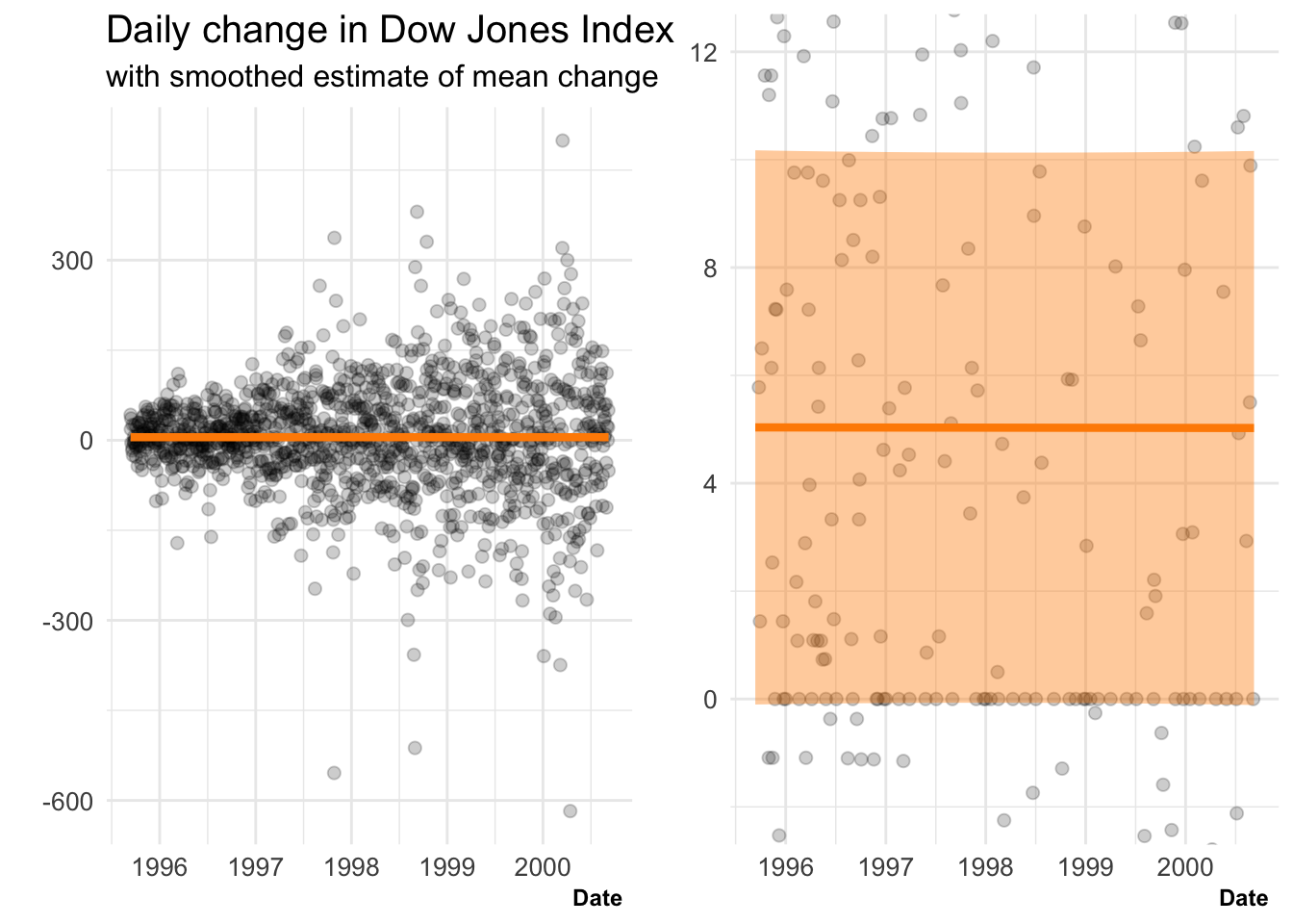
Some degree of statistical rigour can be added to EDA through the use of non-parametric techniques; methods like rolling averages, smoothing or partitioning can to help identify trends or patterns while making minimal assumptions about the data generating process.
Daily change in Dow Jones Index with smoothed estimate of mean and 95% confidence interval.
Code
knitr::kable( x =dowjones%>%mutate(index_change =Index-lag(Index))%>%mutate(after_june_98 =Date>as.Date("1998-06-01"))%>%group_by(after_june_98)%>%summarise( mean =mean(index_change, na.rm =TRUE), sd =sd(index_change, na.rm =TRUE)), caption ="Mean and standard deviation of daily change in Dow Jones Index, before and after 1st of June 1998.")
Mean and standard deviation of daily change in Dow Jones Index, before and after 1st of June 1998.
after_june_98
mean
sd
FALSE
5.916798
65.19093
TRUE
3.972929
119.56067
Though the assumptions in an EDA are often minimal it can help to make them explicit. For example, in this plot a moving averages is shown with a confidence band, but the construction of this band makes the implicit assumption that, at least locally, our observations have the same distribution and so are exchangeable.
Finally, EDA is not a prescriptive process. While I have given a lot of suggestions on what you might usually want to consider, there is no correct way to go about an EDA because it is so heavily dependent on the particular dataset, its interpretation and the task you want to achieve with it. This is one of the parts of data science that make it a craft that you hone with experience, rather than an algorithmic process. When you work in a particular area for a long time you develop domain-specific knowledge of common data quirks, which may or may not translate to other applications.
Now that we have a better idea of what is and what is not EDA, let’s talk about the issue that an EDA tries to resolve and the other issues that it generates.
8.7 Issue: Forking Paths
In any data science project you have to make a sequence of very many decisions, each with many potential options. It is almost impossible to anticipate all of the decisions you will have to make ahead of time and even more difficult do decide how to proceed with each decision a priori.
Focusing in on only one small part of the data science process, we might consider picking a null or baseline model that we will then try and improve on. Should that null model make constant predictions, incorporate a simple linear trend or is something more flexible obviously needed? Do you have the option to try all of these or are you working under time constraints? Is there any domain knowledge that rules some of these null models out on contextual grounds?
An EDA lets you narrow down your options by looking at your data and helps you to decide what might be reasonable modelling approaches.
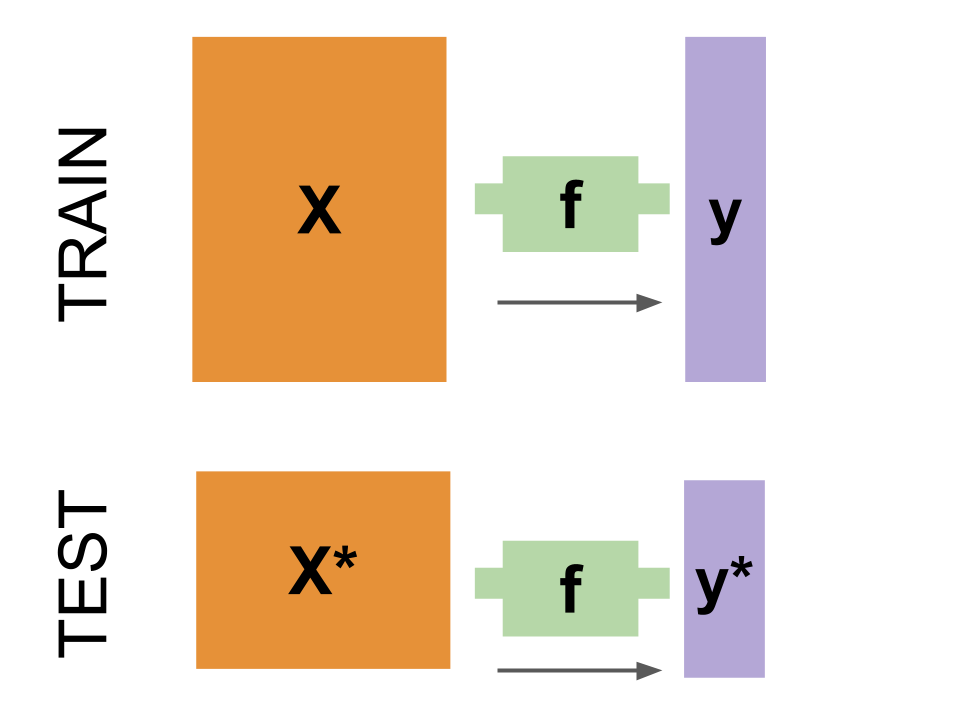
The problem that sneaks in here is data leakage. Formally this is where training data is included in test set but this sort of information leak can happen informally too. Usually this is because you’ve seen the data you’re trying to model or predict and then selected your modelling approach based on that information.
Standard, frequentist statistical methods for estimation and testing assume no “peeking” of this type has occurred. If we use these methods without acknowledging that we have already observed our data then we will artificially inflate the significance of our findings. For example, we might be comparing two models: the first of which makes constant predictions with regard to a predictor, while the second includes a linear trend. We will of course use a statistical test to confirm that what we are seeing is unlikely by chance. However, we must be aware this test was only performed because we had previously examined at the data and noticed what looked to be a trend.
Similar issues arise in Bayesian approaches, particularly when constructing or eliciting prior distributions for our model parameters. One nice thing that we can do in the Bayesian setting is to simulate data from the prior predictive distribution and then get an expert to check that these datasets seem seem reasonable. However, it is often the case this expert is also the person who collected the data we will soon be modelling. It’s very difficult for them to ignore what they have seen, which leads to similar, subtle leakage problems. (For further discussion see the relevant sections of Gelman et al. (2020) or Betancourt (2020))
8.8 Correction Methods
There are various methods or corrections that we can apply during our testing and estimation procedures to ensure that our error rates or confidence intervals account for our previous “peeking” during EDA.
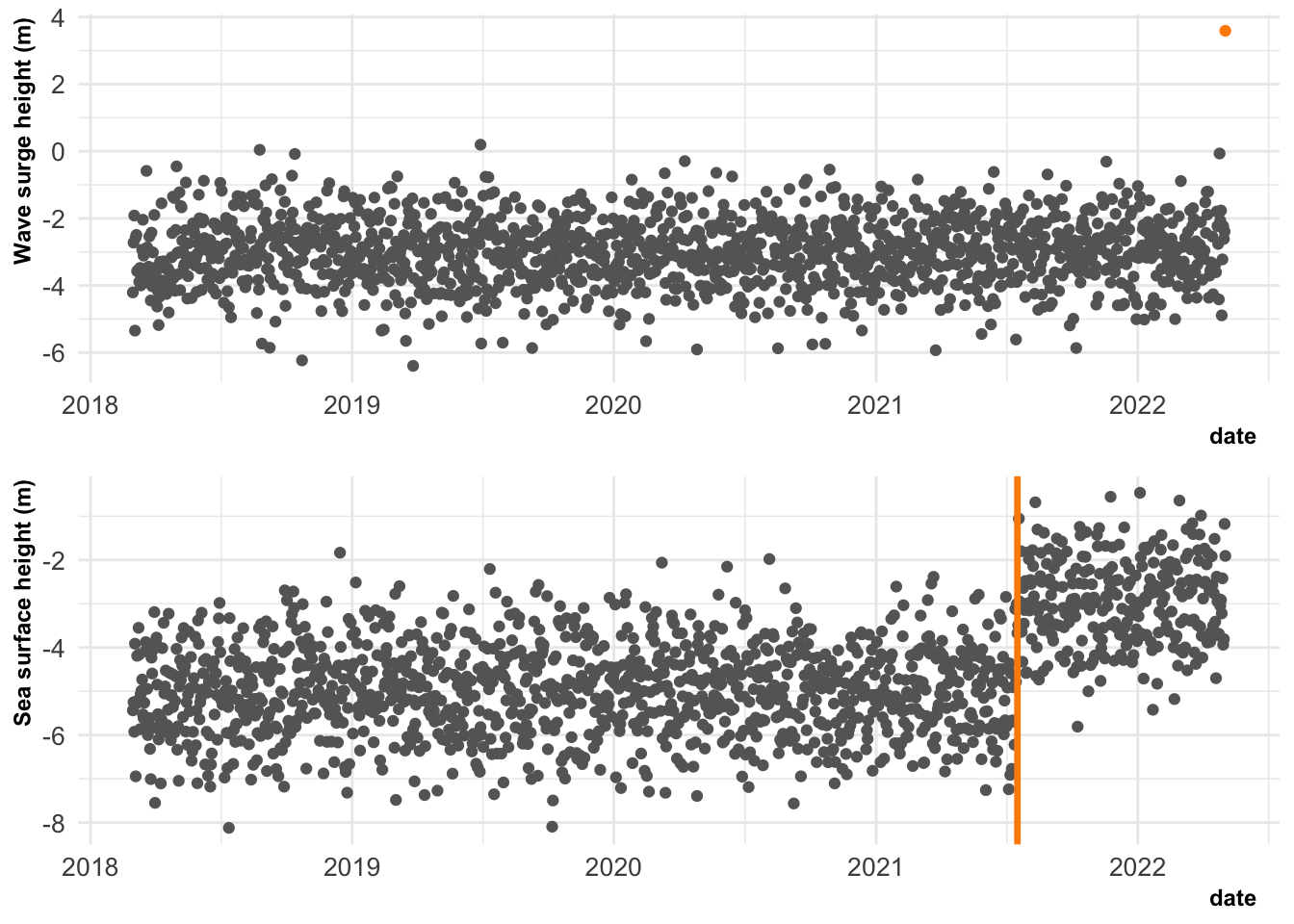
Examples of these corrections have been developed across many fields of statistics. In medical statistics we have approaches like the Bonferroni correction, to account for carrying out multiple hypothesis tests. In the change-point literature there are techniques for estimating a change location given that a change has been detected somewhere in a time series. While in the extreme value literature there are methods to estimate the required level of protection against rare events, given that the analysis was triggered by the current protections having been compromised.
Example sea-height datasets where an analysis has been triggered by an extreme value (above) or a visually identified change in mean (below).
All of these corrections require us to make assumptions about the nature of the peeking. They are either very specific about the process that has occurred, or else are very pessimistic about how much information has been leaked. Developing such corrections to account for EDA isn’t really possible, given its adaptive and non-prescriptive nature.
In addition to being either highly specific or pessimistic, these corrections can also be hard to derive and complicated to implement. This is why in settings where the power of tests or level of estimation is critically important, the entire analysis is pre-registered. In clinical trials, for example, every step of the analysis is specified before any data are collected. In data science this rigorous approach is rarely taken.
As statistically trained data scientists, it is important for us to remain humble about our potential findings and to suggest follow up studies to confirm the presence of any relationships we do find.
8.9 Learning More
In this chapter we have acknowledged that exploratory analyses are an important part of the data science workflow; this is true not only for us as data scientists, but also for the other people who are involved with our projects. We’ve also seen that an exploratory analysis can help to guide the progression of our projects, but that in doing so we must take care to prevent and acknowledge the risk of data leakage.
If you want to explore this topic further, it can be quite challenging. Examples of good, exploratory data analyses can be difficult to come by because, unlike the papers and technical reports that they precede, exploratory analyses are not often made publicly available. Additionally, they are often kept out of public repositories because they are not as “polished” as the rest of the project. Personally, I think this is a shame and the culture on this is slowly changing.
For now, your best approach to learning about what makes a good exploratory analysis is to do lots of your own and to talk to you colleagues about their approaches. There are lots of list-articles out there claiming to give you a comprehensive list of steps for any exploratory analysis. These can be good for inspiration, but I strongly advise you against falling into the trap of treating these as prescriptive or foolproof.
Despite the name of the chapter, Roger Peng’s EDA check-list gives an excellent worked example of an exploratory analysis in R. In discussion article “Exploratory Data Analysis for Complex Models”, Andrew Gelman makes a more abstract discussion of both exploratory analyses (which happen before modelling) and confirmatory analyses (which happen afterwards).